PyTorch for Deep Learning & Machine Learning – Full Course(3) - NoTe0x008
原链接:
https://www.youtube.com/watch?v=V_xro1bcAuA
写在前面
这一系列是我在学习他人的优质课程(博客文章、视频课程等)时所做的学习笔记,根据我自身的水平来进行学习,同时会进行思维的发散,补充原文中没有提到或者有错误的地方。同时也会进行经常性的更新和整理,让它和我的当下的状态更加契合。
这是Free Camp在油管中的PyTorch教程的第三期,我们主要来学习视频中Chapter2的部分。这一部分是在学习如何用神经网络来完成分类问题。
利用circle的二分类问题
Introduction to machine learning classification
分类问题是预测某个对象属于哪一类的任务。首先我们先制造一些数据吧。
1
2
3
4
5
6
7
8
9
10
11
12
13
14
15
16
17
18
19
20
21
| import torch
import sklearn
from sklearn.datasets import make_circles
n_samples = 1000
X, y = make_circles(n_samples,noise=0.03,random_state=42)
print(f"First 5 samples of X:\n {X[:5]}")
print(f"First 5 samples of y:\n {y[:5]}")
|
获得了数据之后,我们利用pandas将其做成一个dataframe,方便我们来进行查看和使用。
1
2
3
4
5
6
7
8
9
10
11
12
13
14
15
16
17
18
19
20
| import pandas as pd
circles = pd.DataFrame({"X1": X[:, 0], "X2": X[:, 1],"label": y})
circles.head(10)
circles.label.value_counts()
|
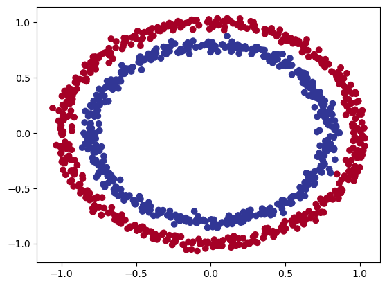
可以看出,外圈和内圈各生成了500个点。为了便于观察,我们将这些点进行可视化看一下,结果如下图所示。作者说,我们所使用的数据通常被称为玩具数据集,这类数据集规模较小,便于快速实验,同时又足够完整,适合用来练习深度学习的基础流程。
1
2
3
| import matplotlib.pyplot as plt
plt.scatter(x=X[:, 0],y=X[:, 1],c=y,cmap=plt.cm.RdYlBu);
|
 由于图片比例的关系,这个圆看起来就没有那么的圆
1
2
3
4
| X.shape, y.shape
type(X), X.dtype
|
现在X和y还是numpy数组,而不是张量,因此我们还得先将他们整理成张量。
1
2
3
4
5
6
7
8
9
10
11
12
|
X = torch.from_numpy(X).type(torch.float)
y = torch.from_numpy(y).type(torch.float)
X[:5], y[:5]
type(X), X.dtype, y.dtype
|
然后利用sklearn.model_selection.train_test_split函数可以将这些数据分为对应的训练集和测试集。
1
2
3
4
5
6
| from sklearn.model_selection import train_test_split
X_train, X_test, y_train, y_test = train_test_split(X, y,test_size=0.2, random_state=42)
len(X_train), len(X_test), len(y_train), len(y_test)
|
Architecture of a classification neural network
这些数据都处理好了之后,我们就可以开始创建模型了。还记得上一章讲的模型最重要的要素吗:结构、损失函数、优化器,以及训练和测试过程。
1
2
3
4
5
| import torch
from torch import nn
device = "cuda" if torch.cuda.is_available() else "mps" if torch.mps.is_available() else "cpu"
device
|
现在就到了创建模型的时间。首先,一个模型需要继承自nn.Module,然后从模型设计来说,该模型需要两个nn.Linear层,使其能适配我们的数据形状。同时别忘了定义对应的forward方法。
1
2
3
4
5
6
7
8
9
10
11
12
13
14
15
16
17
18
19
20
21
22
23
| from sklearn import datasets
class CircleModelV0(nn.Module):
def __init__(self):
super().__init__()
self.layer_1 = nn.Linear(in_features=2, out_features=5)
self.layer_2 = nn.Linear(in_features=5, out_features=1)
def forward(self, x):
return self.layer_2(self.layer_1(x))
model_0 = CircleModelV0().to(device)
model_0
|
Using torch.nn.Sequential
除了上述手动定义的方式,nn.Sequential可以让我们快速构建模型,而无需手动编写forward()方法。
1
2
3
4
5
6
7
8
9
10
11
12
13
14
15
16
17
18
19
20
21
| model_0 = nn.Sequential(
nn.Linear(in_features=2, out_features=5),
nn.Linear(in_features=5, out_features=1)
).to(device)
model_0
model_0.state_dict()
|
直接让他做预测看看。
1
2
3
4
5
6
7
8
9
10
11
12
13
14
15
16
17
18
19
20
21
22
23
| with torch.inference_mode():
untrained_preds = model_0(X_test.to(device))
len(untrained_preds),untrained_preds.shape
len(X_test),X_test.shape
torch.round(untrained_preds[:10])
y_test[:10]
|
Loss, optimizer and evaluation functions for classification
在分类问题中,我们通常选择的损失函数是二元交叉熵(Binary Cross Entropy)或者分类交叉熵(Categorical Cross Entropy,即普通交叉熵)。而我们使用的优化器一般是随机梯度下降(SGD)或者Adam。
在这里我们使用的损失函数是nn.BCEWithLogicalLoss。
1
2
3
4
5
6
7
8
| loss_fn = nn.BCEWithLogitsLoss()
optimizer = torch.optim.SGD(params=model_0.parameters(),lr=0.1)
def accuracy_fn(y_true, y_pred):
correct = torch.eq(y_true, y_pred).sum().item()
acc = (correct/len(y_pred)) * 100
return acc
|
Train and test loops
别忘了一个训练循环包括以下步骤:
- 前向传播
- 计算损失
- 优化器清零梯度
- 损失反向传播
- 优化器更新参数
我们模型输出的是原始对数几率(logits)可以通过将其传入某种激活函数来将其转换为预测概率(例如,二分类使用Sigmoid,多分类使用Softmax),然后可以通过四舍五入或者argmax将预测概率转换为预测标签。
1
2
3
4
5
6
7
8
9
10
11
12
13
14
15
16
17
18
| model_0.eval()
with torch.inference_mode():
y_logits = model_0(X_test.to(device))[:5]
y_logits
y_pred_probs = torch.sigmoid(y_logits)
y_pred_probs
|
对于我们预测的概率值,直接进行区间取整处理。
y_pred_probs >= 0.5时,y=1。y_pred_probs < 0.5时,y=0。
1
2
3
4
5
6
7
|
y_preds = torch.round(y_pred_probs)
y_pred_labels = torch.round(torch.sigmoid(model_0(X_test.to(device))[:5]))
y_preds.squeeze(), y_pred_labels.squeeze()
|
接下来构建对应的训练代码。
1
2
3
4
5
6
7
8
9
10
11
12
13
14
15
16
17
18
19
20
21
22
23
24
25
26
27
28
29
30
31
32
33
34
35
36
37
38
| torch.manual_seed(42)
torch.cuda.manual_seed(42)
epochs = 100
X_train, y_train = X_train.to(device), y_train.to(device)
X_test, y_test = X_test.to(device), y_test.to(device)
for epoch in range(epochs):
model_0.train()
y_logits = model_0(X_train).squeeze()
y_pred = torch.round(torch.sigmoid(y_logits))
loss = loss_fn(y_logits, y_train)
acc = accuracy_fn(y_true=y_train, y_pred=y_pred)
optimizer.zero_grad()
loss.backward()
optimizer.step()
model_0.eval()
with torch.inference_mode():
test_logits = model_0(X_test).squeeze()
test_pred = torch.round(torch.sigmoid(test_logits))
test_loss = loss_fn(test_logits,y_test)
test_acc = accuracy_fn(y_true=y_test,y_pred=test_pred)
if epoch % 10 == 0:
print(f"Epoch: {epoch} | Loss: {loss:.5f}, Acc: {acc:.2f}% | Test loss: {test_loss:.5f}, Test acc: {test_acc:.2f}%")
|
输出如下。
1
2
3
4
5
6
7
8
9
10
| Epoch: 0 | Loss: 0.71773, Acc: 50.00% | Test loss: 0.72110, Test acc: 50.00%
Epoch: 10 | Loss: 0.70335, Acc: 50.00% | Test loss: 0.70843, Test acc: 50.00%
Epoch: 20 | Loss: 0.69769, Acc: 54.75% | Test loss: 0.70326, Test acc: 55.50%
Epoch: 30 | Loss: 0.69539, Acc: 54.00% | Test loss: 0.70094, Test acc: 51.00%
Epoch: 40 | Loss: 0.69440, Acc: 52.75% | Test loss: 0.69973, Test acc: 49.00%
Epoch: 50 | Loss: 0.69392, Acc: 52.12% | Test loss: 0.69895, Test acc: 47.00%
Epoch: 60 | Loss: 0.69365, Acc: 51.88% | Test loss: 0.69837, Test acc: 46.50%
Epoch: 70 | Loss: 0.69348, Acc: 51.38% | Test loss: 0.69789, Test acc: 46.50%
Epoch: 80 | Loss: 0.69337, Acc: 50.88% | Test loss: 0.69749, Test acc: 47.00%
Epoch: 90 | Loss: 0.69328, Acc: 51.38% | Test loss: 0.69714, Test acc: 47.50%
|
Discussing options to improve a model
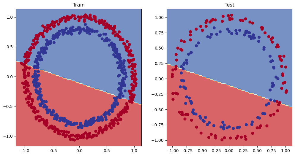
这个概率我说实话,似乎就像是没有学到任何东西,准确率和直接随机预测似乎没有区别,为了做一些深入检查我们需要将它们进行可视化。
1
2
3
4
5
6
7
8
9
10
| from helper_functions import plot_predictions, plot_decision_boundary
plt.figure(figsize=(12, 6))
plt.subplot(1, 2, 1)
plt.title("Train")
plot_decision_boundary(model_0, X_train, y_train)
plt.subplot(1, 2, 2)
plt.title("Test")
plot_decision_boundary(model_0, X_test, y_test)
|
可视化显示的图片如图所示。
说实话我看不出这个图片有什么用
要改进一个模型,我们都有什么方法呢?
- 增加层数,为模型提供更多学习的机会。
- 增加隐藏层神经元数量,例如从5个增加到10个。
- 延长训练时间,增加epoch的数量。
- 更换激活函数,尝试不同的非线性激活函数。
- 调整学习率,改变优化器更新参数的步长。
- 更换损失函数,尝试不同的损失计算方式。
这些都是模型视角的调整,直接作用于模型本身,而非数据层面,都是我们可以手动调整的,被称作超参数。现在我们增加网络层数、增加训练论述,以及增加隐藏层的单元数,尝试使用我们的V1版模型。
1
2
3
4
5
6
7
8
9
10
11
12
13
14
15
16
17
18
19
20
21
22
23
24
25
26
27
28
29
30
31
32
33
34
35
36
37
38
39
40
41
42
43
44
45
46
47
48
49
50
51
52
53
54
55
56
57
58
59
60
61
62
63
64
| class CircleModelV1(nn.Module):
def __init__(self):
super().__init__()
self.layer_1 = nn.Linear(in_features=2, out_features=10)
self.layer_2 = nn.Linear(in_features=10, out_features=10)
self.layer_3 = nn.Linear(in_features=10, out_features=1)
def forward(self, x):
return self.layer_3(self.layer_2(self.layer_1(x)))
model_1 = CircleModelV1().to(device)
model_1
loss_fn = nn.BCEWithLogitsLoss()
optimizer = torch.optim.SGD(params=model_1.parameters(), lr=0.1)
torch.manual_seed(42)
torch.cuda.manual_seed(42)
epochs = 100
X_train, y_train = X_train.to(device), y_train.to(device)
X_test, y_test = X_test.to(device), y_test.to(device)
for epoch in range(epochs):
model_1.train()
y_logits = model_1(X_train).squeeze()
y_pred = torch.round(torch.sigmoid(y_logits))
loss = loss_fn(y_logits, y_train)
acc = accuracy_fn(y_true=y_train, y_pred=y_pred)
optimizer.zero_grad()
loss.backward()
optimizer.step()
model_1.eval()
with torch.inference_mode():
test_logits = model_1(X_test).squeeze()
test_pred = torch.round(torch.sigmoid(test_logits))
test_loss = loss_fn(test_logits,y_test)
test_acc = accuracy_fn(y_true=y_test,y_pred=test_pred)
if epoch % 10 == 0:
print(f"Epoch: {epoch} | Loss: {loss:.5f}, Acc: {acc:.2f}% | Test loss: {test_loss:.5f}, Test acc: {test_acc:.2f}%")
|
我说实话这个效果也一般。
1
2
3
4
5
6
7
8
9
10
| Epoch: 0 | Loss: 0.69396, Acc: 50.88% | Test loss: 0.69261, Test acc: 51.00%
Epoch: 100 | Loss: 0.69305, Acc: 50.38% | Test loss: 0.69379, Test acc: 48.00%
Epoch: 200 | Loss: 0.69299, Acc: 51.12% | Test loss: 0.69437, Test acc: 46.00%
Epoch: 300 | Loss: 0.69298, Acc: 51.62% | Test loss: 0.69458, Test acc: 45.00%
Epoch: 400 | Loss: 0.69298, Acc: 51.12% | Test loss: 0.69465, Test acc: 46.00%
Epoch: 500 | Loss: 0.69298, Acc: 51.00% | Test loss: 0.69467, Test acc: 46.00%
Epoch: 600 | Loss: 0.69298, Acc: 51.00% | Test loss: 0.69468, Test acc: 46.00%
Epoch: 700 | Loss: 0.69298, Acc: 51.00% | Test loss: 0.69468, Test acc: 46.00%
Epoch: 800 | Loss: 0.69298, Acc: 51.00% | Test loss: 0.69468, Test acc: 46.00%
Epoch: 900 | Loss: 0.69298, Acc: 51.00% | Test loss: 0.69468, Test acc: 46.00%
|
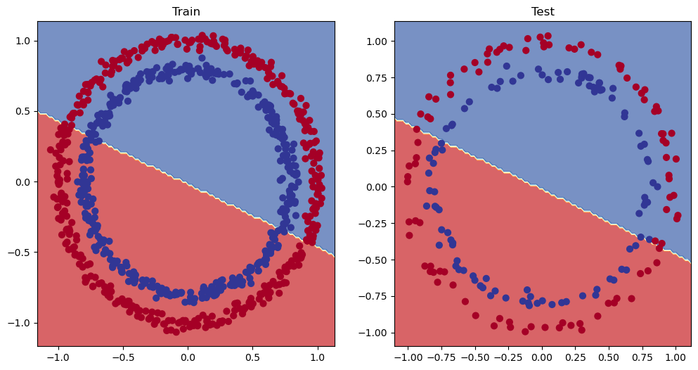
画图出来看一下,还是刚才的图片代码。
1
2
3
4
5
6
7
8
| from helper_functions import plot_predictions, plot_decision_boundary
plt.figure(figsize=(12, 6))
plt.subplot(1, 2, 1)
plt.title("Train")
plot_decision_boundary(model_1, X_train, y_train)
plt.subplot(1, 2, 2)
plt.title("Test")
plot_decision_boundary(model_1, X_test, y_test)
|
除了背景斜率有点区别之外我感觉都差不多
Creating a straight line dataset
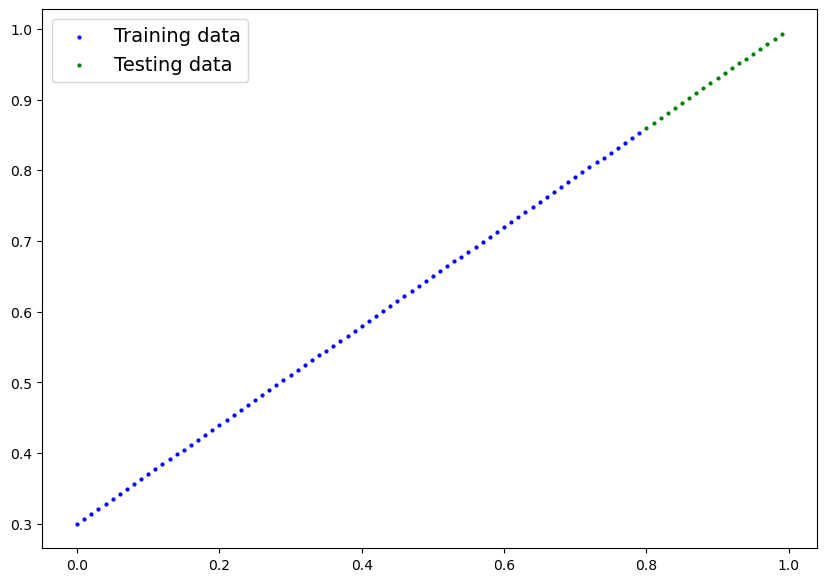
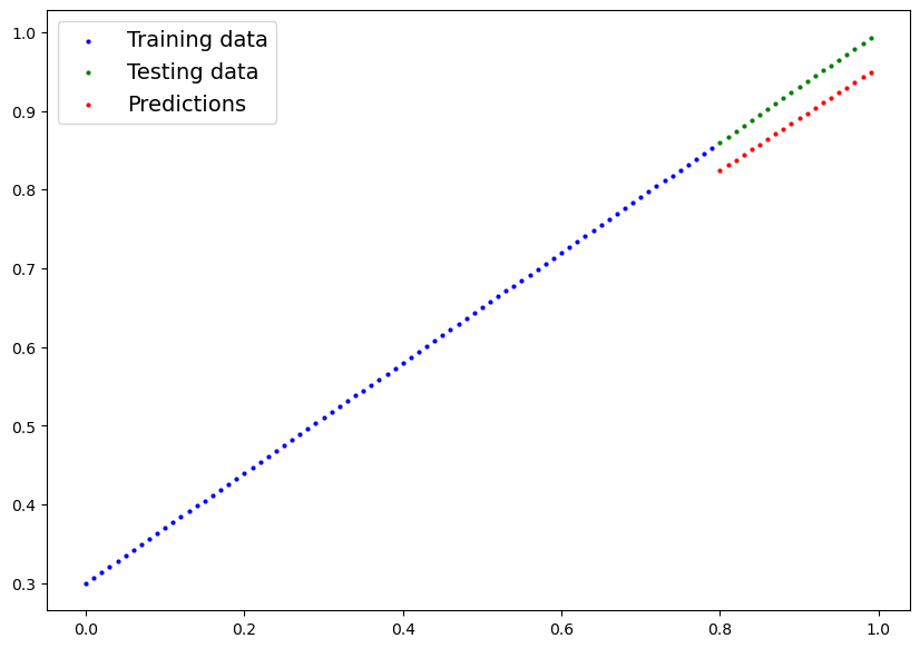
都差不多,那么我们就需要排查排查了。最有效的方法是准备一个小问题看看他能不能办得到。也就是我们需要再次用上一回的那个直线数据集了。
1
2
3
4
5
6
7
8
9
10
11
12
13
14
15
16
17
18
19
20
21
22
23
24
25
26
27
28
|
weight = 0.7
bias = 0.3
start = 0
end = 1
step = 0.01
X_regression = torch.arange(start, end, step).unsqueeze(dim=1)
y_regression = weight * X_regression + bias
X_regression[:5], y_regression[:5]
train_split = int(0.8 * len(X_regression))
X_train_regression, y_train_regression = X_regression[:train_split], y_regression[:train_split]
X_test_regression, y_test_regression = X_regression[train_split:], y_regression[train_split:]
len(X_train_regression), len(X_test_regression), len(y_train_regression), len(y_test_regression)
plot_predictions(train_data=X_train_regression, train_labels=y_train_regression,test_data=X_test_regression,test_labels=y_test_regression)
|
感觉这个图比上次的大多了
Evaluating our model’s predictions
为了测试我们的模型到底有没有问题,我们仿照model_1的结构,设置一个其它参数一样只是输入输出有区别的model_2来进行测试。
1
2
3
4
5
6
7
8
9
10
11
12
13
14
15
16
17
18
19
20
21
22
23
24
25
26
27
28
29
30
31
32
33
34
35
36
37
38
39
40
| model_2 = nn.Sequential(
nn.Linear(in_features=1, out_features=10),
nn.Linear(in_features=10, out_features=10),
nn.Linear(in_features=10, out_features=1)
).to(device)
model_2
loss_fn = nn.L1Loss()
optimizer = torch.optim.SGD(params=model_2.parameters(), lr=0.01)
torch.manual_seed(42)
torch.cuda.manual_seed(42)
epochs = 1000
X_train_regression, y_train_regression = X_train_regression.to(device), y_train_regression.to(device)
X_test_regression, y_test_regression = X_test_regression.to(device), y_test_regression.to(device)
for epoch in range(epochs):
y_pred = model_2(X_train_regression)
loss = loss_fn(y_pred, y_train_regression)
optimizer.zero_grad()
loss.backward()
optimizer.step()
model_2.eval()
with torch.inference_mode():
test_pred = model_2(X_test_regression)
test_loss = loss_fn(test_pred, y_test_regression)
if epoch % 100 == 0:
print(f"Epoch: {epoch} | Loss: {loss:.5f} | Test loss: {test_loss:.5f}")
model_2.eval()
with torch.inference_mode():
y_preds = model_2(X_test_regression)
plot_predictions(train_data=X_train_regression.cpu(), train_labels=y_train_regression.cpu(),test_data=X_test_regression.cpu(),test_labels=y_test_regression.cpu(),predictions=y_preds.cpu());
|
1
2
3
4
5
6
7
8
9
10
| Epoch: 0 | Loss: 0.75986 | Test loss: 0.91103
Epoch: 100 | Loss: 0.02858 | Test loss: 0.00081
Epoch: 200 | Loss: 0.02533 | Test loss: 0.00209
Epoch: 300 | Loss: 0.02137 | Test loss: 0.00305
Epoch: 400 | Loss: 0.01964 | Test loss: 0.00341
Epoch: 500 | Loss: 0.01940 | Test loss: 0.00387
Epoch: 600 | Loss: 0.01903 | Test loss: 0.00379
Epoch: 700 | Loss: 0.01878 | Test loss: 0.00381
Epoch: 800 | Loss: 0.01840 | Test loss: 0.00329
Epoch: 900 | Loss: 0.01798 | Test loss: 0.00360
|
再可视化一下结果看看:
感觉结果也不太对
The missing piece – non-linearity
到底哪里出了问题呢?实际上就是我们的非线性函数不够多。我们现在更新一下我们的类,让他在每一层处理中间添加一个非线性的激活函数,创建一个模型model_3。
1
2
3
4
5
6
7
8
9
10
11
12
13
14
15
16
17
18
19
20
21
22
23
24
25
26
27
28
29
30
31
32
33
34
35
36
37
38
39
40
41
42
43
44
45
46
47
48
49
50
51
52
53
54
55
56
57
58
59
60
61
62
63
| from torch import nn
class CircleModelV2(nn.Module):
def __init__(self):
super().__init__()
self.layer_1 = nn.Linear(in_features=2, out_features=10)
self.layer_2 = nn.Linear(in_features=10, out_features=10)
self.layer_3 = nn.Linear(in_features=10, out_features=1)
self.relu = nn.ReLU()
def forward(self, x):
return self.layer_3(self.relu(self.layer_2(self.relu(self.layer_1(x)))))
model_3 = CircleModelV2().to(device)
model_3
loss_fn = nn.BCEWithLogitsLoss()
optimizer = torch.optim.SGD(model_3.parameters(), lr=0.1)
torch.manual_seed(42)
torch.cuda.manual_seed(42)
epochs = 1000
X_train, y_train = X_train.to(device), y_train.to(device)
X_test, y_test = X_test.to(device), y_test.to(device)
for epoch in range(epochs):
model_3.train()
y_logits = model_3(X_train).squeeze()
y_pred = torch.round(torch.sigmoid(y_logits))
loss = loss_fn(y_logits, y_train)
acc = accuracy_fn(y_true=y_train, y_pred=y_pred)
optimizer.zero_grad()
loss.backward()
optimizer.step()
model_3.eval()
with torch.inference_mode():
test_logits = model_3(X_test).squeeze()
test_pred = torch.round(torch.sigmoid(test_logits))
test_loss = loss_fn(test_logits,y_test)
test_acc = accuracy_fn(y_true=y_test,y_pred=test_pred)
if epoch % 10 == 0:
print(f"Epoch: {epoch} | Loss: {loss:.5f}, Acc: {acc:.2f}% | Test loss: {test_loss:.5f}, Test acc: {test_acc:.2f}%"
|
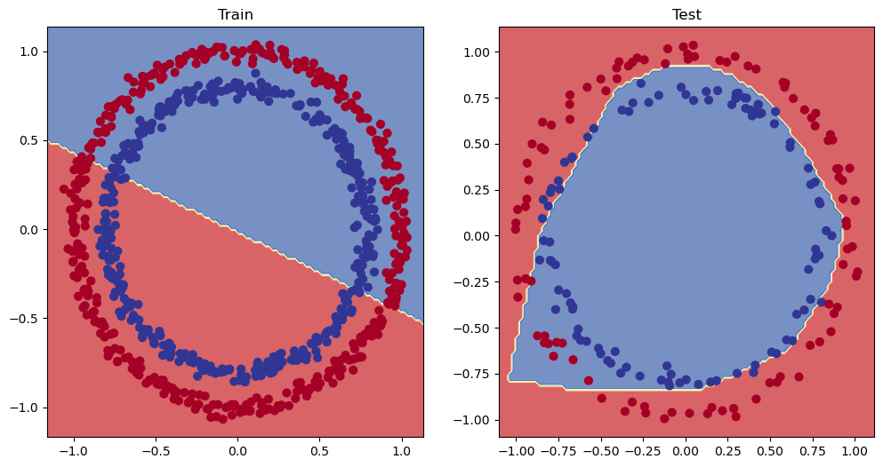
最后这个准确率看起来似乎达到了要求,画图看一下吧。
1
2
3
4
5
6
7
8
9
| plt.figure(figsize=(12, 6))
plt.subplot(1, 2, 1)
plt.title("Train")
plot_decision_boundary(model_1, X_train, y_train)
plt.subplot(1, 2, 2)
plt.title("Test")
plot_decision_boundary(model_3, X_test, y_test)
|
你要是这样的话那我大概能看出来这个图是干嘛的
同时作者问我们,能不能尝试让模型在测试集上的准确率达到80%以上呢?
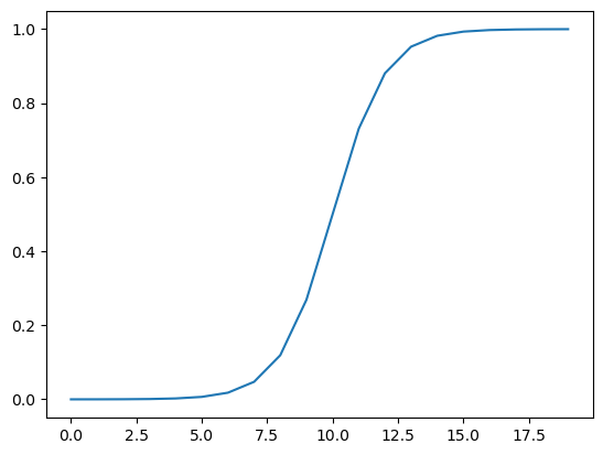
对于神经网络,我们并不明确告知模型该学习什么,而是赋予其工具,让它能自主发掘数据中的模式与规律,这些工具便是线性与非线性函数。
1
2
3
4
5
6
7
8
9
| A = torch.arange(-10, 10, 1, dtype=torch.float32)
A
torch.relu(A)
torch.sigmoid(A)
|
这样直接看sigmod说实话看着太费劲了,我们把它可视化一下。
看起来很像酸碱中和滴定时候的ph值变化
Putting it all together with a multiclass problem
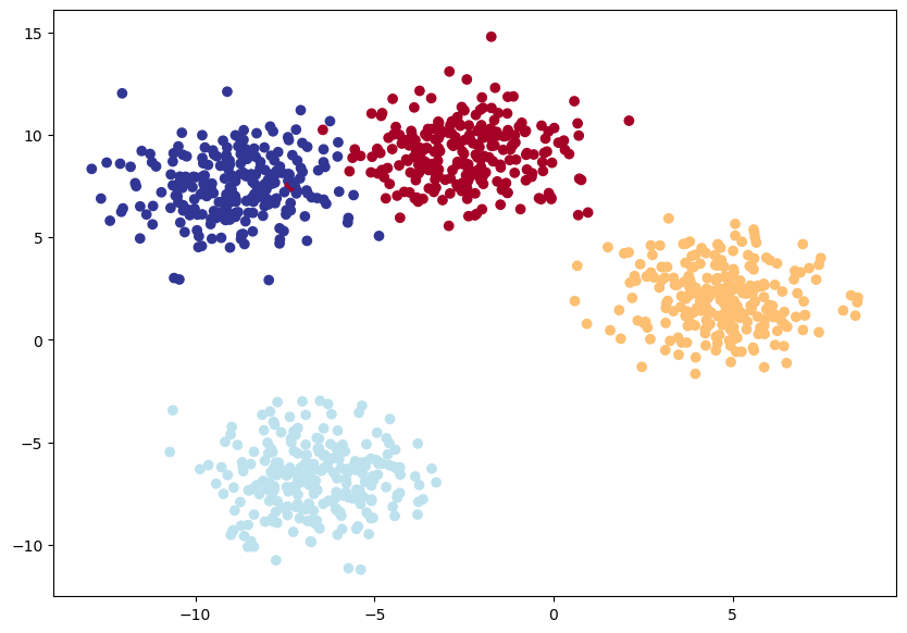
接下来我们尝试进行一个多分类问题,区别于传统的猫狗大战,这种多分类问题并不是非此即彼的选择,有很多个类别要用,例如猫狗还是鸡。首先我们依旧获取一些数据。
1
2
3
4
5
6
7
8
9
10
11
12
13
14
15
16
17
18
19
20
21
22
23
| import torch
import matplotlib.pyplot as plt
from sklearn.datasets import make_blobs
from sklearn.model_selection import train_test_split
NUM_CLASSES = 4
NUM_FEATURES = 2
RANDOM_SEED = 42
X_blob, y_blob = make_blobs(n_samples=1000,n_features=NUM_FEATURES,centers=NUM_CLASSES, cluster_std=1.5, random_state= RANDOM_SEED, return_centers=False)
X_blob = torch.from_numpy(X_blob).type(torch.float32)
y_blob = torch.from_numpy(y_blob).type(torch.int64)
X_blob_train, X_blob_test, y_blob_train, y_blob_test = train_test_split(X_blob,y_blob,test_size=0.2,random_state=RANDOM_SEED)
plt.figure(figsize=(10,7))
plt.scatter(X_blob[:,0],X_blob[:,1],c=y_blob,cmap=plt.get_cmap("RdYlBu"))
|
这个图颇有我上学期做数学建模的意思了
接下来我们就可以创建对应的模型了。我们的模型包括三层线性层,每一层之间都用一个ReLU激活函数。
1
2
3
4
5
6
7
8
9
10
11
12
13
14
15
16
17
18
19
20
21
22
23
24
25
26
| from torch import nn
device = "cuda" if torch.cuda.is_available() else "mps" if torch.mps.is_available() else "cpu"
class BlobModel(nn.Module):
def __init__(self, input_features, output_features, hidden_units=8):
super().__init__()
self.linear_layer_stack = nn.Sequential(
nn.Linear(in_features=input_features, out_features=hidden_units),
nn.ReLU(),
nn.Linear(in_features=hidden_units, out_features=hidden_units),
nn.ReLU(),
nn.Linear(in_features=hidden_units, out_features=output_features)
)
def forward(self,x):
return self.linear_layer_stack(x)
model_4 = BlobModel(input_features=2, output_features=4, hidden_units=8).to(device)
model_4
|
然后就是定义损失函数、优化器以及编写训练代码,这里的损失函数以及优化器都是比较适合多分类任务的。
1
2
3
4
5
6
7
8
9
10
11
12
13
14
15
16
17
18
19
20
21
22
23
24
25
26
27
28
29
30
31
32
33
| epochs = 100
X_blob_train, y_blob_train = X_blob_train.to(device), y_blob_train.to(device)
X_blob_test, y_blob_test = X_blob_test.to(device), y_blob_test.to(device)
for epoch in range(epochs):
model_4.train()
y_logits = model_4(X_blob_train)
y_pred = torch.softmax(y_logits,dim=1).argmax(dim=1)
loss = loss_fn(y_logits,y_blob_train)
accrancy = accuracy_fn(y_true=y_blob_train, y_pred=y_pred)
optimizer.zero_grad()
loss.backward()
optimizer.step()
model_4.eval()
with torch.inference_mode():
test_logits = model_4(X_blob_test)
test_preds = torch.softmax(test_logits,dim=1).argmax(dim=1)
test_loss = loss_fn(test_logits, y_blob_test)
test_acc = accuracy_fn(y_true=y_blob_test, y_pred=test_preds)
if epoch %10 ==0:
print(f"Epoch: {epoch},Loss: {loss:.4f}, Acc: {accrancy:.2f}, Test Loss: {test_loss:.4f}, Test acc: {test_acc:.2f}%")
|
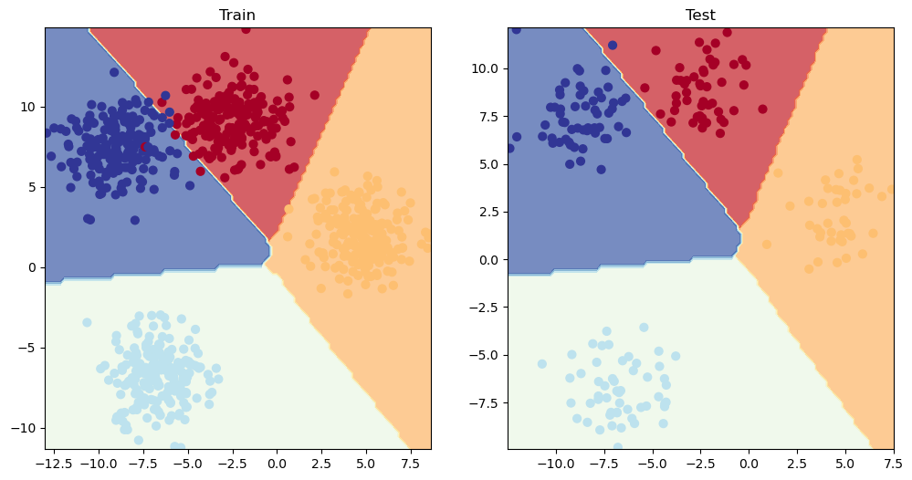
这个效果真的是出奇的好,直接让他画图来看看效果吧。
1
2
3
4
5
6
7
| plt.figure(figsize=(12, 6))
plt.subplot(1, 2, 1)
plt.title("Train")
plot_decision_boundary(model_4, X_blob_train, y_blob_train)
plt.subplot(1, 2, 2)
plt.title("Test")
plot_decision_boundary(model_4, X_blob_test, y_blob_test)
|
这个边界分的非常的准确我说实话
作者同时还给我们介绍了一些其他的判断训练结果的方法,例如混淆矩阵,混淆矩阵是一个N*N(N是类别数)的表格,用于展示模型预测结果与真实标签之间的关系。
总结
在这一个Chapter中,我们学习了如何创建一个分类任务专用的神经网络,同时也掌握了更多的优化模型的方法。感觉很多神经网络的代码似乎都能看得懂了这下。